The Business Objective
This is a case study project. The task is to perform analysis for “Bellabeats”, a technology company made to help women have more accessible knowledge to their health and well being. Goals of this project are to gain insight into Bellabeats smart device product usage for the purpose of guiding the marketing team to a well-informed decision for targeting new potential users.
Analysis Tools
The tool I will be using is the R programming language. It possesses a huge library for data analysis and deep, articulate tools for data visualization. I also enjoy using programming languages for the fine control and maneuverability they offer with data sets.
Libraries used
    library(tidyverse)
    library(dplyr)
    library(janitor)
    library(lubridate)
    library(ggplot2)
    library(skimr)
    library(tidyr)
Imported Datasets
I’ve imported two datasets exported from the Fitbit Tracker Kaggle Page. One dataset spans 03-25-2016 to 04-1216, the other 04-12-2016 to 05-12-2016. The CSV files were imported into R while appending _March-April and _April-May respectively.
    dailyActivity_April_May <- read_csv("Fitabase Data 4.12.16-5.12.16/dailyActivity_merged.csv")
    dailyActivity_March_April <- read_csv("Fitabase Data 4.12.16-5.12.16/dailyActivity_merged.csv")
    heartrate_seconds_merged_April_May <- read_csv("Fitabase Data 4.12.16-5.12.16/heartrate_seconds_merged.csv")
    hourlyCalories_merged_April_May <- read_csv("Fitabase Data 4.12.16-5.12.16/hourlyCalories_merged.csv")
    hourlyCalories_merged_March_April <- read_csv("Fitabase Data 3.12.16-4.11.16/hourlyCalories_merged.csv")
    hourlyIntensities_merged_April_May <- read_csv("Fitabase Data 4.12.16-5.12.16/hourlyIntensities_merged.csv")
    hourlyIntensities_merged_March_April <- read_csv("Fitabase Data 3.12.16-4.11.16/hourlyIntensities_merged.csv")
    hourlySteps_merged_April_May <- read_csv("Fitabase Data 4.12.16-5.12.16/hourlySteps_merged.csv")
    hourlySteps_merged_March_April <- read_csv("Fitabase Data 3.12.16-4.11.16/hourlySteps_merged.csv")
    minuteSleep_merged_April_May <- read_csv("Fitabase Data 4.12.16-5.12.16/minuteSleep_merged.csv")
    minuteSleep_merged_March_April <- read_csv("Fitabase Data 3.12.16-4.11.16/minuteSleep_merged.csv")
    sleepDay_April_May <- read_csv("Fitabase Data 4.12.16-5.12.16/sleepDay_merged.csv")
    weightLogInfo_merged_April_May <- read_csv("Fitabase Data 4.12.16-5.12.16/weightLogInfo_merged.csv")
    weightLogInfo_merged_March_April <- read_csv("Fitabase Data 3.12.16-4.11.16/weightLogInfo_merged.csv")
    "etc ..."

    ## [1] "etc ..."
Formatting
After inspecting the data I decided that appending the two different data sets where my next priority. Running glimpse on the data sets, I discovered the issue of the Date being a “chr” type instead of “Date” type on all the tables. (Note I had already renamed variables and removed the prior ones, hence the new name)
    glimpse(dailyActivity_April_May)

    ## Rows: 940
    ## Columns: 15
    ## $ Id                       <dbl> 1503960366, 1503960366, 1503960366, 150396036…
    ## $ ActivityDate             <chr> "4/12/2016", "4/13/2016", "4/14/2016", "4/15/…
    ## $ TotalSteps               <dbl> 13162, 10735, 10460, 9762, 12669, 9705, 13019…
    ## $ TotalDistance            <dbl> 8.50, 6.97, 6.74, 6.28, 8.16, 6.48, 8.59, 9.8…
    ## $ TrackerDistance          <dbl> 8.50, 6.97, 6.74, 6.28, 8.16, 6.48, 8.59, 9.8…
    ## $ LoggedActivitiesDistance <dbl> 0, 0, 0, 0, 0, 0, 0, 0, 0, 0, 0, 0, 0, 0, 0, …
    ## $ VeryActiveDistance       <dbl> 1.88, 1.57, 2.44, 2.14, 2.71, 3.19, 3.25, 3.5…
    ## $ ModeratelyActiveDistance <dbl> 0.55, 0.69, 0.40, 1.26, 0.41, 0.78, 0.64, 1.3…
    ## $ LightActiveDistance      <dbl> 6.06, 4.71, 3.91, 2.83, 5.04, 2.51, 4.71, 5.0…
    ## $ SedentaryActiveDistance  <dbl> 0, 0, 0, 0, 0, 0, 0, 0, 0, 0, 0, 0, 0, 0, 0, …
    ## $ VeryActiveMinutes        <dbl> 25, 21, 30, 29, 36, 38, 42, 50, 28, 19, 66, 4…
    ## $ FairlyActiveMinutes      <dbl> 13, 19, 11, 34, 10, 20, 16, 31, 12, 8, 27, 21…
    ## $ LightlyActiveMinutes     <dbl> 328, 217, 181, 209, 221, 164, 233, 264, 205, …
    ## $ SedentaryMinutes         <dbl> 728, 776, 1218, 726, 773, 539, 1149, 775, 818…
    ## $ Calories                 <dbl> 1985, 1797, 1776, 1745, 1863, 1728, 1921, 203…

    glimpse(hourlyCalories_merged_April_May)

    ## Rows: 22,099
    ## Columns: 3
    ## $ Id           <dbl> 1503960366, 1503960366, 1503960366, 1503960366, 150396036…
    ## $ ActivityHour <chr> "4/12/2016 12:00:00 AM", "4/12/2016 1:00:00 AM", "4/12/20…
    ## $ Calories     <dbl> 81, 61, 59, 47, 48, 48, 48, 47, 68, 141, 99, 76, 73, 66, …
A common issue with imported data. I corrected the type using lubridates
mdy() function on that variable and all the other ones for
consistency.
dailyActivity_April_May$ActivityDate <- mdy(dailyActivity_April_May$ActivityDate)
dailyActivity_March_April$ActivityDate <- mdy(dailyActivity_March_April$ActivityDate)
formatting for the data frames with hours and minutes was also performed and made easy using lubridate.
    hourlyCalories_merged_April_May$ActivityHour <- mdy_hms(hourlyCalories_merged_April_May$ActivityHour)
    hourlyCalories_merged_March_April$ActivityHour <- mdy_hms(hourlyCalories_merged_March_April$ActivityHour)
    hourlyIntensities_merged_April_May$ActivityHour <- mdy_hms(hourlyIntensities_merged_April_May$ActivityHour)
    hourlyIntensities_merged_March_April$ActivityHour <- mdy_hms(hourlyIntensities_merged_March_April$ActivityHour)
    hourlySteps_merged_April_May$ActivityHour <- mdy_hms(hourlySteps_merged_April_May$ActivityHour)
    hourlySteps_merged_March_April$ActivityHour <- mdy_hms(hourlySteps_merged_March_April$ActivityHour)
    minuteSleep_merged_April_May$date <- mdy_hms(minuteSleep_merged_April_May$date)
    minuteSleep_merged_March_April$date <- mdy_hms(minuteSleep_merged_March_April$date)
    sleepDay_April_May$SleepDay <- mdy_hms(sleepDay_April_May$SleepDay)
    weightLogInfo_merged_April_May$Date <- mdy_hms(weightLogInfo_merged_April_May$Date)
    weightLogInfo_merged_March_April$Date <- mdy_hms(weightLogInfo_merged_March_April$Date)
Also filled in the N/A values for the fat column on the weightLogInfo data sets.
    weightLogInfo_merged_April_May <- weightLogInfo_merged_April_May %>% replace_na(list(Fat = 0))
    weightLogInfo_merged_March_April <- weightLogInfo_merged_March_April %>% replace_na(list(Fat = 0))
Narrowing focus
After imported the data I decided to narrow my focus to variables that
suited the task and appended the split data sets into variable per
tracking category. Id decided to use dailyActivites, weightMerged,
hourlyCalories, hourlyIntensities, and hourlySteps And I removed
unecessary data sets and duplicates with distinct() that wouldn’t
serve insights. This way we have a slightly larger data set and the data
more centralized which will allow a smoother analysis. While also
providing the variables more readability of course.
    dailyActivity <- bind_rows(dailyActivity_March_April, dailyActivity_April_May) %>%
      distinct(Id, ActivityDate, .keep_all = TRUE) %>%
      # 3. Optional: Sort by ID and Date to ensure chronological order
      arrange(Id, ActivityDate)

    n_distinct(dailyActivity$Id)

    ## [1] 33

    weightMerged <- bind_rows(weightLogInfo_merged_March_April, weightLogInfo_merged_April_May) %>%
      distinct(Id, Date, .keep_all = TRUE) %>%
      semi_join(dailyActivity, by = "Id") %>%
      arrange(Id, Date)

    n_distinct(weightMerged$Id)

    ## [1] 12

    hourlyCalories <- bind_rows(hourlyCalories_merged_March_April, hourlyCalories_merged_April_May) %>%
      distinct(Id, ActivityHour, .keep_all = TRUE) %>%
      semi_join(dailyActivity, by = "Id") %>%

      arrange(Id, ActivityHour)

    n_distinct(hourlyCalories$Id)

    ## [1] 33

    hourlyIntensities <- bind_rows(hourlyIntensities_merged_March_April, hourlyIntensities_merged_April_May) %>%
      distinct(Id, ActivityHour, .keep_all = TRUE) %>%
      semi_join(dailyActivity, by = "Id") %>%
      arrange(Id, ActivityHour)

    n_distinct(hourlyIntensities$Id)

    ## [1] 33

    hourlySteps <- bind_rows(hourlySteps_merged_March_April, hourlySteps_merged_April_May) %>%
      distinct(Id, ActivityHour, .keep_all = TRUE) %>%
      semi_join(dailyActivity, by = "Id") %>%
      arrange(Id, ActivityHour)

    n_distinct(hourlySteps$Id)

    ## [1] 33

    # n_distinct(sleepDay_April_May$Id)
We have 33 Ids for dailyActivity which equals the amount stated is
present in the data set. For the rest of the values I used semi-join
to only merge with Ids present in dailyActivity.
Quick Data Summaries
I ran summary all the individual variables filtering out 0s, assuming they were a lack of input, for quick insights and accurate calculations
# Summary data
    dailyActivity %>% select(TotalSteps,
                             TotalDistance,
                             Calories,
                             LoggedActivitiesDistance,
                             VeryActiveDistance,
                             VeryActiveMinutes,
                             ModeratelyActiveDistance,
                             FairlyActiveMinutes,
                             LightActiveDistance,
                             LightlyActiveMinutes,
                             SedentaryMinutes
                             ) %>%
      mutate(across(everything(), ~na_if(., 0))) %>%
      summary()


    ##    TotalSteps    TotalDistance       Calories    LoggedActivitiesDistance
    ##  Min.   :    4   Min.   : 0.010   Min.   :  52   Min.   :1.960
    ##  1st Qu.: 4923   1st Qu.: 3.373   1st Qu.:1834   1st Qu.:2.092
    ##  Median : 8053   Median : 5.590   Median :2144   Median :2.253
    ##  Mean   : 8319   Mean   : 5.986   Mean   :2313   Mean   :3.178
    ##  3rd Qu.:11092   3rd Qu.: 7.905   3rd Qu.:2794   3rd Qu.:4.864
    ##  Max.   :36019   Max.   :28.030   Max.   :4900   Max.   :4.942
    ##  NA's   :77      NA's   :78       NA's   :4      NA's   :908
    ##  VeryActiveDistance VeryActiveMinutes ModeratelyActiveDistance
    ##  Min.   : 0.020     Min.   :  1.00    Min.   :0.010
    ##  1st Qu.: 0.595     1st Qu.: 10.00    1st Qu.:0.340
    ##  Median : 1.760     Median : 27.00    Median :0.660
    ##  Mean   : 2.680     Mean   : 37.47    Mean   :0.963
    ##  3rd Qu.: 3.530     3rd Qu.: 55.00    3rd Qu.:1.200
    ##  Max.   :21.920     Max.   :210.00    Max.   :6.480
    ##  NA's   :413        NA's   :409       NA's   :386
    ##  FairlyActiveMinutes LightActiveDistance LightlyActiveMinutes SedentaryMinutes
    ##  Min.   :  1.00      Min.   : 0.010      Min.   :  1.0        Min.   :   2.0
    ##  1st Qu.:  8.00      1st Qu.: 2.365      1st Qu.:148.0        1st Qu.: 730.0
    ##  Median : 16.00      Median : 3.590      Median :209.5        Median :1058.0
    ##  Mean   : 22.93      Mean   : 3.673      Mean   :211.7        Mean   : 992.3
    ##  3rd Qu.: 30.00      3rd Qu.: 4.905      3rd Qu.:272.0        3rd Qu.:1230.0
    ##  Max.   :143.00      Max.   :10.710      Max.   :518.0        Max.   :1440.0
    ##  NA's   :384         NA's   :85          NA's   :84           NA's   :1
weightMerged %>% select(WeightKg, WeightPounds, BMI, IsManualReport) %>%
     mutate(across(everything(), ~na_if(., 0))) %>%
     summary()

   ##     WeightKg      WeightPounds        BMI        IsManualReport
   ##  Min.   : 52.6   Min.   :116.0   Min.   :21.45   Mode:logical
   ##  1st Qu.: 61.5   1st Qu.:135.6   1st Qu.:24.00   TRUE:62
   ##  Median : 62.5   Median :137.8   Median :24.39   NA's:35
   ##  Mean   : 72.3   Mean   :159.4   Mean   :25.38
   ##  3rd Qu.: 85.1   3rd Qu.:187.6   3rd Qu.:25.59
   ##  Max.   :133.5   Max.   :294.3   Max.   :47.54

   hourlyCalories %>% select(Calories) %>%
     mutate(across(everything(), ~na_if(., 0))) %>%
     summary()

   ##     Calories
   ##  Min.   : 42.00
   ##  1st Qu.: 62.00
   ##  Median : 82.00
   ##  Mean   : 96.09
   ##  3rd Qu.:106.00
   ##  Max.   :948.00

   hourlyIntensities %>% select(TotalIntensity, AverageIntensity) %>%
     mutate(across(everything(), ~na_if(., 0))) %>%
     summary()

   ##  TotalIntensity   AverageIntensity
   ##  Min.   :  1.00   Min.   :0.0167
   ##  1st Qu.:  5.00   1st Qu.:0.0833
   ##  Median : 13.00   Median :0.2167
   ##  Mean   : 20.22   Mean   :0.3370
   ##  3rd Qu.: 25.00   3rd Qu.:0.4167
   ##  Max.   :180.00   Max.   :3.0000
   ##  NA's   :19360    NA's   :19360

   hourlySteps %>% select(StepTotal) %>%
     mutate(across(everything(), ~na_if(., 0))) %>%
     summary()

   ##    StepTotal
   ##  Min.   :    1.0
   ##  1st Qu.:   95.0
   ##  Median :  273.5
   ##  Mean   :  545.8
   ##  3rd Qu.:  639.8
   ##  Max.   :10565.0
   ##  NA's   :19811

   sleepDay_April_May %>% select(TotalMinutesAsleep, TotalTimeInBed) %>%
     mutate(across(everything(), ~na_if(., 0))) %>%
     summary()

   ##  TotalMinutesAsleep TotalTimeInBed
   ##  Min.   : 58.0      Min.   : 61.0
   ##  1st Qu.:361.0      1st Qu.:403.0
   ##  Median :433.0      Median :463.0
   ##  Mean   :419.5      Mean   :458.6
   ##  3rd Qu.:490.0      3rd Qu.:526.0
   ##  Max.   :796.0      Max.   :961.0
The following observations were made specifically with women in mind:
-
Average Sedimentary minutes is extremely high. Users are wearing their device outside of activities.
-
Daily activities like Moderately Active Distance and Fairly Active Minutes for users are low. Users aren’t wearing their devices for medium intensity exercise or may not be tracking them.
-
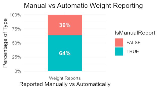
Over 50% of reporting is done manually. This number should be reduced or streamlined for easier and simplistic health journalism.
-
Users spend roughly 7 hours asleep a night and an extra 30 in bed. Users wear their devices frequently to bed, must be comfortable and un-impeding devices?
Users are wearing their devices for a majority of the day and not just for exercise. Having extensive tracking data for metrics like intense exercise, sleeping and even high sedimentary minutes insinuate that users devices must be comfortable and that they wear them for very long periods of time. Another metric that is telling is ** manual reporting ** for exercise. Users dont rely on the fit bit to track every exercise per say but they do rely on the storing and analyzing of their reported data. Another sign of that is the Weight Logs metrics.
Data Viz
Below will show how long the user wears their device i.e. how much they use it. Health habits data is useful in this case but it truly serve to represent product usage over time in this report.
Average Daily Activity
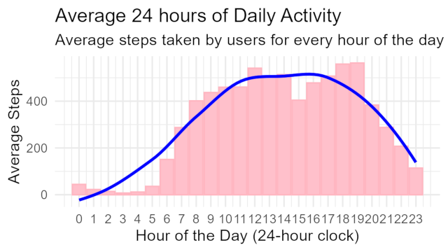
Below we see that users steps increase on either the commute to work or it could be exercise at 8-9 A.M. Normally numbers drop between 9AM and 5PM due to work but we actually see higher amounts of steps between the “Work Valley” hours. Users seem are tracking alot of steps in between these hours. Insight: Users are tracking their steps throughout the day. This also means their wearing them all day. Marketing angle: “Bellabeats makes wear for style and health”
average24HoursStepsViz <- hourlySteps %>%
  mutate("Hour" = hour(ActivityHour)) %>%
  group_by(Hour) %>%
  summarize(AverageSteps = mean(StepTotal, na.rm = TRUE))
High Sedimentary hours
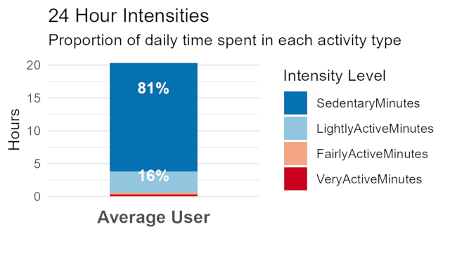
High sedimentary minutes means the user is more than likely sitting or lying down, or not moving around very much. This shows that a large number of users use these devices even though they don’t have very high “VeryActiveMinutes” metrics (less than 5%). Insight: These products are being worn for more than just fitness tracking. THeir for lifestyle. Marketing angle: “Bellabeats products are for women of every lifestyle”
Average 24 hour Intensities
  summarize(
    VeryActiveMinutes = mean(VeryActiveMinutes, na.rm = TRUE),
    FairlyActiveMinutes = mean(FairlyActiveMinutes, na.rm = TRUE),
    LightlyActiveMinutes = mean(LightlyActiveMinutes, na.rm = TRUE),
    SedentaryMinutes = mean(SedentaryMinutes, na.rm = TRUE)) %>%
  pivot_longer(
    cols=everything(),
    names_to = "ActivityType",
    values_to = "Minutes"
  ) %>%
  mutate(Percentage = Minutes / sum(Minutes),
         Label = scales::percent(Percentage, accuracy = 1)) %>%
  mutate(ActivityType =  factor(ActivityType, levels = c("SedentaryMinutes" ,
                                                         "LightlyActiveMinutes" ,
                                                         "FairlyActiveMinutes",
                                                         "VeryActiveMinutes")))
Health Journaling
Another angle to explore product usage is for users reporting their own entries for weight. Users have reported over 60% of their weight data. Mainly because of most devices do not have scales available. Users are using fit bit as a health journal not just tracking their activities. Giving users clear ownership over data is important to most smart device users. Bella could also benefit from providing users with more health metrics that can be reported as well as more control over their journal habits. It would also be another avenue to deliver specific pieces of knowledge with overwhelming users with a plethora of information that they would have to sift through. Insight: Users are using fit bit as a health journal not just tracking their activities. Marketing angle: “Bellabeats is here to help you with all your health needs.”
## Manual Reporting viz
manualReporting <- weightMerged %>%
  count(IsManualReport) %>%
  mutate(
    Percentage = n / sum(n),
    Label = scales::percent(Percentage, accuracy = 1)
  )